All work was done using ArcGIS v10.1, with a raster (grid) cell size of 100 ft, with elevations in feet relative to NAVD 1988, and X-Y coordinates in the standard State Plane Florida east zone, 1983-HARN, US feet. The extent is X from 205000 to 750000 and Y from 270000 to 1045000, creating a gridded dataset of 5450-by-7750 cells. Almost all of the source data had been previously compiled. The process consisted of assembling the topographic data at 100-ft cell size, layering together the topographic data, blending the source layers to remove discontinuities along the edges, assembling and layering together the bathymetric data, joining the bathymetric with the topographic data, and filling in any remaining no-data holes along the shoreline.
Most of the project land area was covered by modern LiDAR data, which had already been processed to create DEMs at 100-ft cell size. Several areas lie in the western zone, and they had already been projected for the Florida east zone. The LiDAR data includes:
- FDEM 2007 Coastal LiDAR project, with partial or complete coverage by county: Lee, Charlotte, Sarasota, Collier, Monroe, and Miami-Dade.
- SWFWMD 2005 LiDAR: Peace River South project, covering part of Charlotte County.
- USGS 2012 LiDAR: Eastern Charlotte project, covering part of eastern Charlotte and western Glades counties.
- USACE 2007 LiDAR: The HHD_EAA project as an add-on to the FDEM Coastal LiDAR project, covering part of Hendry, Glades, Palm Beach, and Okeechobee counties. The USACE also processed and merged in bathymetric data from Lake Okeechobee (from USGS and other boat surveys) at 100-ft cell size.
- USACE 2010 LiDAR: The HHD_Northwest dataset was merged from two deliverables named HHD NW Shore and Fisheating Creek, and covers parts of Okeechobee, Glades, Highlands, and Charlotte counties.
- USACE 2003 LiDAR: The Southwest Florida Feasibility Study (SWFFS) LiDAR covered parts of Collier, Hendry, and Glades counties. This dataset has lower quality than the other LiDAR data.
For the Everglades and Big Cypress areas, the collection of LiDAR data is problematic due to extremely dense vegetation cover. The USGS conducted a project through 2007 to collected high-accuracy elevation points throughout those areas, essentially using a plumb bob hanging from a helicopter equipped with GPS. This high-accuracy elevation dataset (HAED) consists of about 50,000 points collected at 400-m intervals. The points were converted to a gridded surface using an ordinary-Kriging interpolation and resampled at 100-ft cell size.
Another problematic area is the well-known “Topo Hole” in SE Hendry and NE Collier counties, where no high-quality elevation data has been collected. Several previous approximations of a topographic surface had been made for this area (2003 and 2005 for the SWFFS, and in early 2006 by the USACE), primarily using 5-ft contours and spot elevations from USGS topographic maps (quad sheets). For this project, several newly available datasets from the C-139 Regional Feasibility Study were obtained, and two were included in the current processing: ground spot-elevations from the “all-static” survey and 1-ft contours for the C-139 Annex area. Unfortunately these new datasets cover only a small area at the margins of the Topo Hole. The contours and spot elevations were converted to a gridded surface using the ArcGIS tool TopoToRaster, formerly known as GridTopo and sometimes referred to as the ANUDEM method, which applies “essentially a discretized thin plate spline technique” to create a “hydrologically correct digital elevation model.” The method is not perfect, and the lack of detailed source data limits the accuracy, but still the result is better than other methods that are currently available. A 20,000-ft buffer zone was added around the Topo Hole, and the TopoToRaster tool was applied. Until LiDAR or similar data is collected for the Topo Hole, this is likely to remain as the best-available approximation of a topographic surface for this area.

 For the Collier, Monroe, and Miami-Dade DEMs, “decorrugated” versions of the processed LiDAR data were used. During the original processing of the accepted deliverables from the FDEM LiDAR project, significant banding was apparent. This banding appears as linear stripes (or corn rows or corrugations) of higher and lower elevations along the LiDAR flightlines. The DEM data can be “decorrugated” by applying a series of filters to the elevation dataset, but real topographic features can also be altered slightly in the process. In the resulting product, the systematic errors are removed, but with the cost that every land elevation is altered to some extent; thus the decorrugated surface is considered a derivative product. The decorrugation work for the rural areas of these three counties was done in 2010, but the results had never been formally documented or added to the District’s GIS Data Catalog. For this project, in comparison with the “original” processed DEMs, these datasets are considered the “best-available” because errors that are visually obvious have been removed.
The best-available topographic DEMs were mosaicked into a single DEM, with better data used in areas of overlap. In order to remove discontinuities where the border of better data joins to other data, a special blending algorithm was used to “feather” the datasets into each other. The result is a surface that is free from discontinuities along the “join” edges, but of course accuracy of the result is limited by the accuracy of the source data. The width of the blending zone along the edges was varied according to the type of data and the amount of overlap that was available, and ranged from 4,000 to 20,000 feet. The “blending-zone” adjusted data was retained and is available for review.
The layering of the topographic data, from best (top) to worst (bottom), is listed here with best listed first:
- 2007 FDEM LiDAR, HHD_EAA, HHD_Northwest, and Eastern Charlotte (all are roughly equivalent in quality)
- SWFWMD 2005 LiDAR
- SWFFS 2003 LiDAR
- USGS HAED
- Topo Hole
As noted above, two datasets for the land area were created. One treated the major lake surfaces as flat areas, and the other used available lake bathymetry to add the lake-bottom elevations into the topo DEM surface. The USACE-processed bathymetry was added for the area of Lake Okeechobee that had been treated as a water body in the 2007 HHD_EAA LiDAR deliverable. Also, bathymetry data for Lake Trafford was available from a 2005 USACE project. In the flat-surface version, elevations of 7.5 ft for Lake Okeechobee and 15.1 ft for Lake Trafford, relative to NAVD 1988, were imposed.
Offshore bathymetry was mosaicked at 100-ft cell size. In 2005 the available data had been collected and mosaicked at 300-ft cell size. Since that time, no significant bathymetry datasets are known to have been created within the Lower West Coast area. In 2004, a best-available composite for the Lee County area had been created at 100-ft cell size from 2002 USACE channel surveys of the Caloosahatchee River, boat surveys by USGS for the Caloosahatchee Estuary in 2003 and other areas in 2004, experimental offshore LiDAR from USGS in 2004, and older NOAA bathymetric data for areas that were not otherwise covered. Other bathymetric data down the shoreline consists of USGS boat surveys down to Cape Romano, Naples Bay boat surveys for SFWMD, and Florida Bay boat surveys that had been compiled in approx. 2004 by Mike Kohler. For the remaining offshore areas, the older NOAA bathymetric data was used. The bathymetric pieces were mosaicked together and blended along their edges.
When the offshore bathymetry was joined with the land topography, there were thousands of small no-data holes near the shoreline. 
These empty spaces were grouped into three categories. First, some small and low-lying islands (essentially mangrove rookeries) in Florida Bay had no pertinent elevation data. These were assigned an arbitrary land elevation of +1.5 ft NAVD88. Secondly, empty spaces adjacent to offshore bathymetry were treated as shallow offshore areas. For each no-data hole (polygon), the maximum elevation for adjacent offshore bathymetry was assigned. (i.e. It’s water, and we’ll give it the shallowest water value that’s nearby). Finally, empty spaces that were inland were treated as low-lying land or marsh. For each no-data hole (polygon), the minimum elevation for adjacent “land” was assigned. (i.e. If it’s a low area, it can’t be above anything that’s along its edge.)
After filling in all of the no-data holes, the bathymetry and land-with-lake topo were mosaicked together. The deepest spot in the full dataset is about 100 ft at a distance of about 90 miles west of Cape Sable. For most modeling and mapping purposes, however, the areas well off the shore (e.g. 10 miles or farther) are not needed. Thus a buffer zone was defined as 20,000 ft beyond the LWC offshore boundary, and the full dataset was clipped to that boundary to create Lwc_TopoShore.

These products can accurately be described as composites of the best-available data. For example, both the 2005 SWF composite and the early-2006 USACE SF-Topo composite were based on older data and did not include any of the LiDAR that was collected after 2003. It might be possible to make slight improvements to the current source data (say, by decorrugating rural Lee County), but such modifications would involve significant time and work that would go beyond the short turn-around time allocated for this project.
Timothy Liebermann, Senior Geographer, Regulation GIS, SFWMD
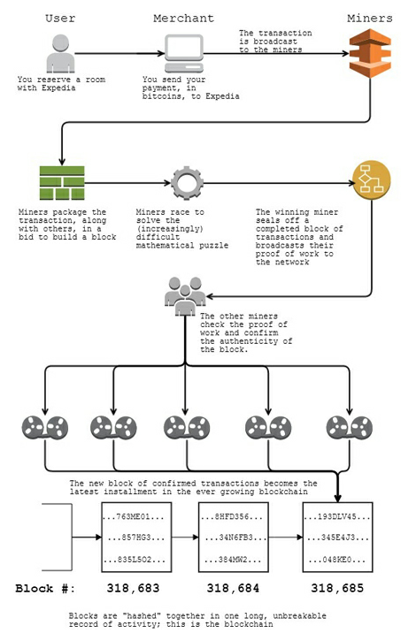
![a-credit-card-payment-is-so-incredibly-simple-until-you-take-a-closer-look[1].png](https://geodemesne.wordpress.com/wp-content/uploads/2017/01/a-credit-card-payment-is-so-incredibly-simple-until-you-take-a-closer-look1.png?w=584)